DEVELOPMENT OF AN ADVANCED ENSEMBLE-BASED OCEAN DATA ASSIMILATION APPROACH FOR OCEAN AND COUPLED REANALYSES
PI and organization: E. de Boisséson (ECMWF)
Co-Is: H. Zuo, M. Balmaseda, P. de Rosnay (ECMWF)
In ocean analysis systems, a substantial part of the uncertainty comes from the observation representativeness errors that are introduced when matching physical observations to the model resolution. The atmospheric forcing and sea surface constraints applied to ocean models are another major source of uncertainty. To reduce problems with representativeness, ocean analysis systems rely on super-observation and thinning techniques to average the information from observations towards the scales of the ocean model. Some of this information is lost in the procedure. The GENOA project delivers a new perturbation method that, together with an ensemble approach, better exploits the information from the observing system.
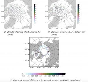
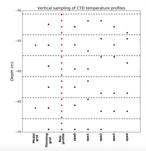
This new method is now implemented in the ECMWF ocean data assimilation system. The perturbation scheme works on both sea surface and subsurface observations. Sea ice concentration data, for example, are usually ingested in the analysis system using a thinning method with a fixed sampling interval (around 0.5 ̊) in both latitudinal and longitudinal directions (Figure 1a). A random sampling method has been imbedded in the thinning scheme (Figure 1b). Together with an ensemble approach, the new scheme uses a greater variety of observation and produces ensemble spread that represent reasonable uncertainties in sea ice concentration (Figure 1c). On the vertical, the current pre-defined vertical thinning scheme (opa0 on Figure 2) has evolved into a random thinning around each thinning level (opa1-to-4 on Figure 2). This method, together with an ensemble approach, allows to exploit the full vertical resolution of the profile observations.
To deal with the uncertainty of the surface forcing, a perturbation repository has been built based on a variety of both atmospheric analysis products and observational-based analyses of surface variables such as Sea Surface Temperature and Sea Ice Concentration. The repository samples the uncertainty at the air- sea interface in various periods to account for the changes in the observing system. The final product of GENOA is a generic ensemble generation scheme that can be applied in both ocean and coupled atmosphere-ocean analysis
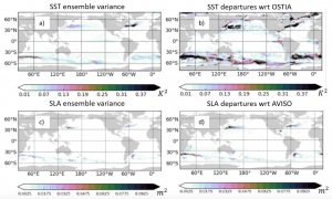
The ensemble generation scheme has been evaluated against observations. Results show that the perturbation method generates physical uncertainty signals. Figure 3a,c shows that the largest uncertainties for surface variables such as SST and Sea Level are in the most energetic and eddy-active areas of the Global Ocean, e.g. the Western Boundary Currents and the Antarctic Circumpolar Current.
The uncertainty signal however remains under-dispersive and overall does not cover for the departures with respect to observations (Figure 3b,d).
The work performed during GENOA is made available to CMEMS MFCs and will serve as a basis for further development of ensemble generation methods for ocean analysis at ECMWF.
Figure 1. (a) Daily-averaged gridded SIC data over the Arctic region from CMEMS OSTIA as assimilated in the ECMWF ORA system using a regular thinning. (b) SIC data as assimilated in the new system using the random thinning method for one specific ensemble member. (c) Ensemble spread of SIC (in %) over the Arctic region in a 5-ensemble member sensitivity experiment using a random sampling of SIC data. As one would expect the uncertainty is more substantial at the sea-ice edge and close to the continent.
Figure 2. Illustration of the vertical sampling method used in the ECMWF ORA system and overview of an alternative method based on a random sampling. From left to right, are plotted the vertical sampling by the model grid between 50m and 70m depth, the standard pre-defined thinning in the ECMWF ORA system (thinning grid), the sampling by a CTD probe (raw profile) and the regular (opa0) and random sampling in four realizations (opa1 to opa4).
Figure 3. a) Ensemble variance of temperature (in ?2); b) root mean squared model departures to CMEMS-OSTIA SST ( in ?2 ); c) ensemble variance of SLA (in ?2 ); b) root mean squared model departures to CMEMS Sea level (in ?2). Ideally, the ensemble variances should match the departures. In this case the ensemble is under-dispersive


