HIGH-RESOLUTION MODEL VERIFICATION EVALUATION
PI and organization: J. Maksymczuk & M. Mittermaier(UK MetOffice)
Co-Is: R. Crocker, C. Pequignet, A. Ryan (UK MetOffice)
The project
The High-resolution model Verification Evaluation (HiVE) project considered CMEMS forecast products applicable to regional domains and aimed to demonstrate, for the first time, the utility of spatial verification methods (originally developed to evaluate km-scale forecasts from atmospheric models), for verifying km-scale ocean model forecasts. It was undertaken to address the need for new metrics adapted to the increased resolution in both observations and models, as identified in the CMEMS Service Evolution Strategy.
Specifics
The project had two key objectives relating to the ongoing assessment protocols for ocean forecast models, and how they could be evolved to cope with future modelling systems. The first part of the project involved evaluating SST forecasts. The second part of the project utilised the Method for Object-based Diagnostic Evaluation (MODE). CMEMS datasets used within the project included:
|
NORTHWESTSHELF_ANALYSIS_FORECAST_PHYS_004_001_b |
AMM7 |
|
NORTHWESTSHELF_ANALYSIS_FORECAST_PHY_004_013 |
AMM15 |
|
IBI_ANALYSIS_FORECAST_PHYS_005_001 |
IBI |
|
NORTHWESTSHELF_ANALYSIS_FORECAST_BIO_004_002_b (v8) |
AMM7v8 |
|
SST_NWS_SST_L4_NRT_OBSERVATIONS_010_003 |
L4-ODYSSEA |
|
INSITU_NWS_NRT_OBSERVATIONS_013_036 |
IN-SITU |
|
OCEANCOLOUR_ATL_CHL_L4_NRT_OBSERVATIONS_009_037 |
L4-multi sensor |
|
NORTHWESTSHELF_ANALYSIS_FORECAST_BIO_004_002_b (v11) |
AMM7v11 BIO DA |
Project highlights
The project has demonstrated that the ocean is very similar to the atmosphere at sub-10 km in that the smaller scale detail is equally noisy, so that coarser resolution models producing smoother forecasts often have better verification results. This is counter-intuitive given that qualitatively the higher-resolution forecasts are more realistic looking. Spatial verification methods can account for apparent mismatch between the quantitative and qualitative outcomes by not expecting the detail to be in the right place at the right time, but to give credit to forecasts being correct “nearby” or “in the vicinity”.
The key findings from the project can be summarised as follows.
For the evaluation of SSTs using HiRA:
- with the application of HiRA it is possible to identify improvements in the higher resolution model which were not apparent using typical grid scale assessments;
- future comparative assessments of ocean models with different resolutions would benefit from using HiRA as part of the evaluation process, as it gives a more equitable and appropriate reflection of model performance at higher resolutions.
A paper on the HiRA findings has been submitted to Ocean Science (Crocker et al. 2020).
For the evaluation of chlorophyll blooms with MODE:
- Bias – there is a significant concentration bias in the forecast compared to the observations, which must be mitigated against before using MODE or MTD; the bias may be improved using a BIO DA analysis to drive the forecast.
- Timing issues – MTD analysis has shown that the initial onset of the bloom is almost a month late (25 days) in AMM7v8. Subsequent events are handled somewhat better.
- Location – beyond the timing issues the model does generally produce chlorophyll objects (blooms) in the right areas, but not necessarily at the right time.
- Evolution with lead time – there is very little change in results between the analysis and the forecasts at all lead times. Predicting the onset of the bloom seems problematic.
- Benefit of AMM7v11 BIO DA – it would be good to see whether forecasts initialised using the BIO DA analysis will improve the timing errors and the bias. The BIO DA analysis is an improvement compared to the one without (which the forecasts in this study were initiated with).
- Size of objects – as for MODE, the objects are generally too large. This spatial extent bias is in addition to the previously mentioned concentration bias.
- Number of objects – AMM7v8 produces fewer objects compared to observed and these are too large. Many of the coastal objects identified in the L4 product cannot be resolved by the model due to the coarseness of the coastline in the 7 km model. This situation would improve should the model resolution increase from 7 km to 1.5 km.
A paper on the MODE and MTD results is in preparation for Ocean Science. Here is a little more detail on the methods and results of the project.
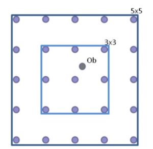
By considering the forecast grid points in predefined neighbourhoods centred on an observing location the methodology utilises ensemble and probabilistic forecast verification metrics such as the Continuous Ranked Probability Score (CRPS, Hersbach 2000). HiRA works on the assumption that all forecast grid points in the neighbourhood, form a pseudo ensemble and are equi- probable outcomes at the observing location.
HiRA – How does it work?
For this assumption to remain true, neighbourhood sizes cannot become too large. The CRPS is an error-based score where a perfect forecast has a score of 0, i.e. smaller scores are better. It measures the difference between two cumulative distributions, a forecast distribution formed by ranking the pseudo-ensemble members in the neighbourhood, and a step function describing the observed state.
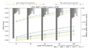
Figure 2 illustrates results obtained from the application of HiRA to the co-located domains of the AMM7 and AMM15 for the period January – December 2019. The lines on the plot show the CRPS obtained from the two configurations as a function of forecast lead time for a number of neighbourhood sizes. Matching line styles represent the equivalent neighbourhood sizes that should be compared.
Figure 2. Summary of CRPS (left axis, lines) and CRPS difference (right axis, bars) for the period January 2019 to December 2019 for the AMM7 and AMM15 co-located model domains at different neighbourhood sizes. The nearest grid point results (labelled 1) are equivalent to the mean absolute error (MAE).
Overall, the results obtained from the application of HiRA suggested that the higher resolution AMM15 consistently had lower errors, indicated here by lower CRPS values, when equivalent neighbourhood extents were compared. The bars are included here to illustrate the differences in the CRPS between the two configurations, where a positive bar implies AMM7 has better (lower) CRPS, and a negative bar implies AMM15 is better. Both configurations show a reduction in error when utilising a neighbourhood compared to using the nearest grid point, suggesting that using a spatial verification method is justified. In addition, sub-setting the data into on-shelf and off-shelf sub-domains demonstrated that different signals can be obtained by isolating different components of the domain. CRPS scores are better for neighbourhoods in the off-shelf sub- domain, where temperatures are spatially smoother. On-shelf the application of neighbourhoods shows a large decrease in error when moving from grid scale to neighbourhood assessment, as small-scale spatial variability becomes encompassed in the scores. In both sub-domains AMM15 has consistently smaller errors. Both models exhibit a worsening of CRPS as the forecast lead time increases, which is more rapid for the off-shelf assessment.
Analysing chlorophyll blooms like objects in space and time
The Method for Object-based Diagnostic Evaluation (MODE) is an object-based verification method. Features or events of interest (called objects) are identified in both a gridded forecast and a gridded ‘truth’ dataset by applying a threshold (which defines the object (Davis et al., 2006). Characteristics or attributes of the forecast and observed objects can then be derived. Forecast and observed objects are also matched or paired up using fuzzy logic so that the attributes of the matched pairs can be analysed, e.g. how close were their centres of mass (centroids), area ratios, distribution of intensities etc. MODE analyses each time slice (in this case daily mean chlorophyll concentration) independently. MODE Time Domain (MTD) on the other hand provides the ability to connect the objects at a given time to those coming before and after, to gain an understanding of how the object (which represents a feature or event of interest) evolves (Mittermaier and Bullock, 2013, Clark et al., 2014). MODE produces 2D space objects, MTD produces 3D space-time objects.
Figure 3 illustrates results obtained from the application of MODE to daily mean chlorophyll forecasts from AMM7 for the 2019 chlorophyll bloom season (March – July, ~150 days) against the cloud-free gridded (L4) daily observations product, and shows the composite spatial coverage of objects identified through the 2019 bloom season for both observed and forecast objects. The maps summarise the proportion of time (in days) that an object occurs at that model grid point. In 3(a), the observed composite, the near continuous presence of chlorophyll near the coasts stands out. Of particular note, there is a patch in the central North Sea where the L4 product has no objects identified but the AMM7 forecasts, 3(b), have objects identified for a low proportion of the time. However, there are areas, for example the south-west approaches, where there appears to be a good level of consistency between the forecast and observed object frequencies.
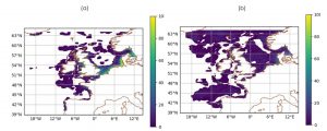 Figure 3: (a) Observed (L4) and (b) AMM7v8 Day 1 object composites for the 2019 bloom season (March – July 2019, inclusive). The colours indicate the proportion of time (in days) that an observed object appears at each grid point.
As well as the products from the CMEMS catalogue, there was also an opportunity to use both MODE and MODE Time Domain (MTD) with analysis data provided from the latest pre- operational AMM7v11 model which includes satellite chlorophyll assimilation (and is due to for Entry Into Service in late 2020). This is referred to here as AMM7v11 BIO DA analysis. To avoid confusion, the non-assimilative biological model is referred to as AMM7v8.
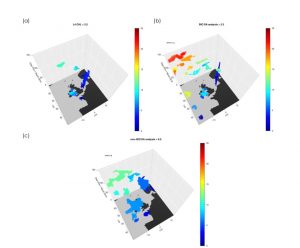
Figure 4: Comparison of the temporal evolution of identified chlorophyll objects using MODE Time Domain (MTD). The evolution is based on the daily sequence of either the L4 satellite product (a), the AMM7v11 BIO DA analysis which includes biogeochemical components (b) and the AMM7v8 analysis without any biogeochemical DA (c). Colours correspond to the object numbers assigned by MTD. Colours represent the object numbers, which increase with time. Thresholds in mg.m-3.
Figure 4 illustrates a summary of the temporal evolution of the chlorophyll blooms during the 2019 season, showing three different analyses: the satellite based L4 product (a), the AMM7v11 BIO DA analysis (b) which assimilates chlorophyll, and the AMM7v8 analysis without any biogeochemical assimilation (c). The assimilation of chlorophyll is sufficient to ensure that the analysis is relatively unbiased (in terms of concentration) compared to the L4 product. Even so the AMM7v11 BIO DA analysis is far more “active” providing many more blooms/episodes. The colours show how the bloom migrates north and west as the season progresses (based on the progression of object identifiers and colours). The non-DA analysis on the other hand produces far fewer blooms/episodes but those that are produced are far too large, suggesting that in addition to the concentration bias there is also a spatial extent bias.
Specific benefits to the CMEMS and the wider community resulting from the HiVE project include:
- a framework that will assess km-scale models appropriately and allow for them to be compared – the HiRA framework has been successfully applied to configurations over a range of scales
- spatial methods that counteract the impact of the double-penalty effect, which acts to destroy the positive signal obtained from the qualitative benefits of km-scale models.
- the metrics used in HiRA can assess both deterministic and ensemble forecasts equitably – HiRA is equally applicable to ensemble forecasts, as it is built around the principle of treating deterministic forecasts like pseudo-ensemble members
- if these types of assessments are run routinely, they can quantify the improvements in forecast skill over time
- tools that can measure the skill of CMEMS products in forecasting events or features of interest in space and time – both MODE and MTD are able to inform users of the timing, extent and duration of coherent structures such chlorophyll blooms as defined by enhanced chlorophyll concentrations.
- introducing and demonstrating the relevance of methods and tools that are used widely within the NWP atmospheric community and applying them to ocean datasets in order to improve the quality assessment of forecast products
References
Clark, A.J., R.G. Bullock, T.L. Jensen, M. Xue, and F. Kong, 2014: Application of Object-Based Time-Domain Diagnostics for Tracking Precipitation Systems in Convection-Allowing Models. Wea. Forecasting, 29, 517– 542, https://doi.org/10.1175/WAF-D-13-00098.1
Crocker, R., Maksymczuk, J., Mittermaier, M.P., Tonani, M., and Pequignet, C., 2020: An approach to the verification of high-resolution ocean models using spatial methods. Submitted to Ocean Science
Davis C.A., B.G. Brown, R.G. Bullock, 2006a: Object-based verification of precipitation forecasts. Part I: methodology and application to mesoscale rain areas. Mon. Weather Rev. 134,1772 – 1784.
Hersbach, H., 2000: Decomposition of the Continuous Ranked Probability Score for Ensemble Prediction Systems. Wea. Forecasting, 15, 559–570, https://doi.org/10.1175.
Mittermaier, M.P., 2014: A strategy for verifying near-convection-resolving forecasts at observing sites. Wea. Forecasting. 29(2), 185-204.
Mittermaier, M.P., and R. Bullock, 2013: Using MODE to explore the spatial and temporal characteristics of cloud cover forecasts from high-resolution NWP models. Meteorol. Apps., 20, 187-196.

