STOCHASTIC COASTAL/REGIONAL UNCERTAINTY MODELLING:
SENSITIVITY, CONSISTENCY AND POTENTIAL CONTRIBUTION TO CMEMS ENSEMBLE DATA ASSIMILATION
PI and organization: Sarantis Sofianos (Univ. of Athens)
Other members of the proposing team: Vassilios Vervatis (Univ. of Athens), Pierre De Mey (CNRS/LEGOS), Nadia Ayoub (CNRS/LEGOS)
External expert involved: George Triantafyllou (HCMR) (DA experts from MO, C.-E. Testut).
Outcome:
The project aimed at strengthening CMEMS in the areas of coastal/regional ocean uncertainty quantification, Ensemble consistency verification and Ensemble data assimilation, designed for the Service Evolution framework within “Lot 3: links with coastal environment”. The work is based on stochastic modelling of ocean physics and biogeochemistry in the Bay of Biscay, on an identical sub-grid configuration of the IBI-MFC system. One important paradigm of this work is to adopt a balanced approach between building Ensembles and testing their relevance. This work is meant to be useful for CMEMS targeted science, for coastal modelling users, but also in general to MFCs and TACs, in particular in the areas of Ensemble-based uncertainty quantification, validation of uncertainty estimates from Ensembles, and Ensemble assimilation capabilities involving physical and biogeochemical variables. Elements available for uptake within CMEMS include numerical modules and toolboxes, as well as Ensembles and reports.
In Task 1, we use stochastic modelling to generate Ensembles describing uncertainties in open ocean and on the shelf, mainly focusing on upper ocean processes. Our stochastic implementation is based on autoregressive processes in the context of the stochastic parameterization of perturbations of the atmosphere-ocean state in the ocean model and of the biogeochemical state in the ecosystem model. The method is complemented to account for spatial correlations and anamorphosis transformation of anisotropic uncertainty patterns, which is of vital importance in high-resolution coastal/regional configurations. Wind uncertainties are found to dominate all other atmosphere-ocean sources of model errors. The Ensemble spread (i.e. 1σ), after one-month spin up period focusing on upper ocean properties, is approximately 0.01 m for SSH and 0.15 °C for SST, though these values vary depending on season and cross shelf regions. In the context of a seasonal Ensemble, the aforementioned values reach close to 0.05 m for SSH and 0.5 °C for SST. Ecosystem model uncertainties emerging from perturbations in physics appear to be moderately larger than those perturbing the concentration of the biogeochemical compartments, resulting in total chlorophyll spread at about 0.01 mg.m-3.
In Task 2, we introduce several methodologies aimed at checking the consistency of the above Ensembles with respect to TAC data and arrays. An Ensemble-based consistency Analysis Toolbox was developed and used to document the statistical consistency of our Ensembles vs. CMEMS data. It will also be delivered to CMEMS groups so that it can be used beyond this project. All Ensembles were found to be underdispersive. Regarding Chl, we identified a statistical biogeochemical spin-up time of the order of 3 months. As a general rule, Ensembles were found to be most consistent in terms of SST, moderately consistent in terms of SLA, and often inconsistent in terms of Chl. We also found that in general Ens-3 (with perturbations in both physics and bgc) was the most consistent. For all variables, pattern consistency was found to be fairly good at the larger scales; it degraded at smaller scales for gridded SLA and for Chl. Some error processes seemed to be missing from the range of perturbations – in particular, some high-frequency error processes are currently unaccounted for on the shelves. We could not clearly attribute the missing processes to any particular error process with the tools at hand. A follow-on proposal (SCRUM2) addresses those questions via probabilistic approaches. The consistency analysis also addressed the question of which routinely-available surface datasets were fit for validating Ensembles. In particular, the use of high-resolution SST products appears necessary when it comes to validating eddy-resolving Ensembles (such as 1/36° here). This is probably also the case for Chl, but is masked at this time by other deficiencies.
In Task 3, we calculated multivariate representers and EnKF incremental analyses from our Ensembles. One objective was to access the impact of observations onto unobserved variables, such as other data types or subsurface variables. The correlation structures revealed general differences between the abyssal and coastal areas, as well as between variables. On the shelves (English Channel and South Armorican shelf), the filament shaped structures for SST, SSS and Chl were likely linked to near-shore features such as river discharges (Loire river plume), mid-shelf thermal fronts and tidal fronts. The effect of spring bloom could be seen on the shelf, confirmed by the negative correlation between SST (e.g., heating up) and Chl (plankton depletion following a bloom). In the abyssal plain, the scales were often characteristic of the underlying quasigeostrophic mesoscale features, Chl included due to the mesoscale vertical velocity field. Most of the Chl correction arise from uncertainties in physics, but bgc model errors tend to enhance the effect of the physics. Logically, assimilating Chl seems to have a very measurable impact on physical variables.
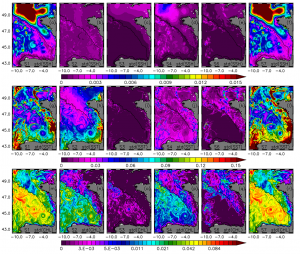
Figure 1. Ensemble spread (i.e. 1σ) daily averaged maps on April 30, 2012 after one month spin-up: (a-f) SSH (m), (g-l) SST (oC) and (m-r) CHL surface concentration (mg/m3). The colorbars are from top to bottom respectively; CHL concentration on logarithmic scale. Sensitivity experiments S1 to S7 are shown from left to right (S5 not shown).
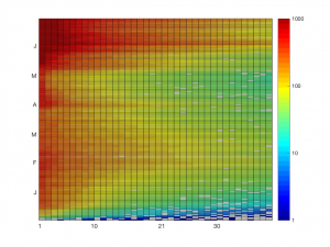
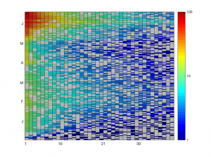
Figure 2. Hovmoller diagram of variations in time of the ArM spectrum, including an OSTIA SST innovation consistency check against Ens-1, projected onto 39 array modes (degrees of freedom calculated out of a 40-member ensemble). White areas depict inconsistent array modes. Colorbar: RM spectrum (values smaller than 1, i.e. dark blue, depict array modes below the observational noise). (a) No decimation. (b) 1/5 decimation (one data point every 5th point retained). Note the different scales in colorbar.
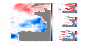
Figure 3. Incremental analysis of the first member assimilating OSTIA-SST1 on May 7, 2012, using Ens1 40 members: (a) correction on SST oC, (b) SSH m, (c) SSS, (d) surface Chl mg/m3.
CMEMS Product ID: 1SST_GLO_SST_L4_NRT_OBSERVATIONS_010_001

